In the old days we were happy with mean field approximation. Currently we don't. As the model goes more complicated, Bayesian inference needs more accurate yet fast approximations to the exact posterior, and apparently mean-field is not a very good choice. To enhance the power of variational approximations people start to use invertible transformations (e.g. see the normalizing flow paper) that warp simple distributions (e.g. factorised Gaussian) to complicated ones that are still differentiable. However it introduces an extra cost: you need to be able to compute the determinant of the Jacobian of that transform in a fast way. Solutions of this include constructing the transform with a sequence of "simple" functions -- simple in the sense that the Jacobian is low-rank or triangular (e.g. see this paper). Recently I found a NIPS preprint that provides another solution of this, which is absolutely amazing: through their clever design you don't even need to compute the Jacobian at all! I found this paper a very interesting read so I decided to put a blog post here:

Stein Variational Gradient Descent: A General Purpose Bayesian Inference Algorithm
Qiang Liu and Dilin Wang
http://arxiv.org/abs/1608.04471 (to appear at NIPS 2016)

You might also want to check out their previous work at this year's ICML.

Before going to the details, let's recap the idea of invertible transformations of random variables. Assume $z$ is a random variable distributed as $q(z)$, e.g. Gaussian. Now if a mapping $T$ is differentiable and invertible, then the transformation $x = T(z)$ is also a random variable, distributed as (using notations in the paper) $q_T(x) = q(T^{-1}(x)) | det(\nabla_x T^{-1}(x)) |$. If we use this distribution in VI, then the variational free energy becomes $\mathrm{KL}[q_T(x)||p(x|\mathcal{D})] - \log p(\mathcal{D})$, which means we need to evaluate the log determinant of the Jacobian $\log | det(\nabla_x T^{-1}(x)) |$. As said $T$ often contains a sequence of "simple" mappings, in math this is $T(z) = F_K(F_{K-1}(...F_1(z)))$, so the determinant term becomes $\sum_{k=1}^K \log |det(\nabla F_k^{-1}) |$.

Previous approaches parameterised the $F$ functions with carefully designed neural networks, and optimised all these network parameters jointly through the free energy. This paper, although not explicitly mentioned, used sequential optimisation instead: it first finds $F_1$ by minimising the energy, then fixes it and proceeds to $F_2$ and so on. No fine-tuning at the end. Now optimisation becomes easier, but potentially you need more transformations and thus longer training time in total. Also storing these functions can be very challenging for memory.

To solve these problems the authors proposed using functional gradients. They assumed a very simple form for the transform: $F_k(z) = z + f_k(z)$ where $f_k$ belongs to some RKHS defined by a kernel $K(x, \cdot)$, and used functional gradients to find the $f_k$ function. Then instead of finding a local optimum of $f_k$, we can do "early stopping", or even just run one gradient step, then move to the next transform. Furthermore, if you start your search at $f_k(z) = 0$, then there's no need to evaluate the determinant as now $\nabla F_{k}^{-1} = I$! This solves the running time problem even when we need much more of these transforms compared to previous approaches. Another nice explanation is that now $T$ becomes $T(z) = z + f(z)$ with $f(z) = \sum_{k=1}^K f_1(z)$, and if the norm of $f_k$ is small enough, then the above is also equivalent to one gradient step for $f$ at point $z + \sum_{i < k} f_i(z)$. I like both ways of interpreting this procedure and I would say it comes from the clever design of the sequential transform.

The authors provided the analytical form of this functional gradient which links back to the kernel Stein discrepancy discussed in their ICML paper:

$\nabla_{f_k} \mathrm{KL}[q_{F_k} || p] |_{f_k = 0} = - \mathbb{E}_{z \sim q} [ \nabla_z K(z, \cdot) + \nabla_z \log p(z) K(z, \cdot) ]$,

where $p(z)$ short-hands the joint distribution $p(z, \mathcal{D})$. Since now Monte Carlo estimation has become quite a standard approach for modern VI, we can use samples from the $q$ distribution to compute the above gradient. Assume we take $n$ samples $z_1, ..., z_n \sim q$. By taking only one gradient step with learning rate $\epsilon$ the current transform becomes $F_k(z) = z + \frac{\epsilon}{n} \sum_n [ \nabla_{z_n} K(z_n, z) + \nabla_{z_n} \log p(z_n) K(z_n, z) ]$. We can also use mini-batches to approximate $\log p(z, \mathcal{D})$ to make the algorithm scalable on large datasets. In fact they reported even faster speed than PBP on Bayesian neural network with comparable results to the state-of-the-art, which looks very promising.

After the gradient step of $f_k$, the algorithm moves to the next transform $F_{k+1}(z) = z + f_{k+1}(z)$ and again starts at $f_{k+1}(z) = 0$. Notice now the $q$ distribution that we simulate $z$ from in the above gradient equation becomes $q_{F_k}$, which do contain a non-identity Jacobian if we want to evaluate it directly. However recall the core idea of invertible transformation that we can simulate $x \sim q_T$ by first sample $z \sim q$ then apply $x = T(z)$, and we do have samples from $q$ from the last step. This means we can first apply the transform to update the samples (with Monte Carlo estimate) $z_i \leftarrow z_i + \frac{\epsilon}{n} \sum_n [ \nabla_{z_n} K(z_n, z_i) + \nabla_{z_n} \log p(z_n) K(z_n, z_i) ]$, then use them to compute this step's gradient. It makes the algorithm sampling-like and the memory consumption only comes from storing these samples, which can be very cheap compared to storing lots of parametric functionals. If one is still unhappy with storing samples (say due to limited memory), one can fit a parametric density to the samples after the last transform $F_K$. Another strategy is to only use 1 sample, and in this case this algorithm reduces to maximum a posteriori (MAP), which still finds a mode of posterior for you.

The authors used RBF kernel and also pointed out that this algorithm also recovers MAP when the bandwidth tends to zero. This make sense as you can understand it through analogies of kernel density estimation, and in general running VI with $q$ as a delta function is also equivalent to MAP. In other words, the number of samples $n$ and the kernel implicitly define the family of variational distribution $q$: the kernel mainly controls the smoothness, and the number of samples roughly indicates the complexity of your fit. Presumably the main criticism I have is also from the nature that $n$ affects the complexity of $q$, which is not the case for other black-box VI techniques. This means in high dimensions where using large number of samples has prohibitive memory cost, you need to carefully tune the kernel parameters in order to get a good fit, or even you might not be able to achieve significantly better results than MAP. Well using mean-field Gaussian in high-dimensions also seems insufficient, but at least the community has relatively clear understanding in this case. For this method it's unclear to me right now what the distribution looks like and whether it is often better than mean-field. Perhaps I should raise this questions to the authors and I’ll be very excited to hear more about it from their poster at NIPS!

We've seem the power of deep learning. But not everyone is happy with just "throwing the dataset to a big neural network". A good model design can still perform well or even better than naive neural network method, but with much fewer number of model parameters. Probabilistic Graphical models (PGMs) method is this type of thing: it has beautiful theory, lots of applications, and many machine learning researchers have been developing models and algorithms based on it. I remember the first deep learning paper I read was about restricted Boltzmann machines (RBM), and today I'm still fascinated by the elegance of the maths.

However inference of PGMs has become the barrier for large scale applications and complicated graphical structure. Surely people have developed fast approximate inference method (VI/EP to name a few) that works very well in practice. But the main problem comes from the memory cost. To make your model powerful you probably want to add a hierarchy of latent variables to describe both local and global behaviour. However for large datasets the number of approximate distribution you need to maintain increases drastically. This is especially true for intermediate-level latent variables (consider topic mixture for each document in LDA for example) which you can't just throw them away in SVI. Perhaps one of the most well known papers to address this problem is Kingma & Welling's variational auto-encoder (VAE), which amortized the inference by learning a mapping (represented by a neural network) from data to local latent variables. Since then this inference network/recognition model idea has been very popular. In this post I'm gonna briefly discuss two recent papers on using neural networks to assist approximate inference which I think are interesting read.

The first paper comes from Ryan Adams group at Harvard:

Composing graphical models with neural networks for structured representations and fast inference
Johnson et al.
https://arxiv.org/pdf/1603.06277v2.pdf

I would say the general idea is very simple: the authors wanted to extend the original SVI method to non-conjugate models. They basically just approximated the non-exponential family likelihood terms with conjugate exponential family distributions, and to reduce memory cost the natural parameters were parameterised by a recognition model. Then you can reuse the SVI derivations to show the fixed point/natural gradient equations, and I think the algorithm can actually be very fast in practice.

I can sort of see why their approach works and in fact I like their recipe which has analytical forms. But the general framework is not that neat: they optimised different objective functions for different parts of variational distribution. It's true that the proposed loss function has the nice lower-bounding property just as SVI, however the authors proved it by saying "the learned local variational distribution using recognition model approximated likelihood terms is not optimal for the exact SVI". In other words, their argument holds for any recognition model, and it's not obvious to me how tight is their objective to the marginal likelihood. But I haven't read the paper in very detail (they have a long appendix) so maybe I'm missing something here.

UPDATE 19/08/16

I actually spent sometime today to read the paper again. Well I still have the above questions. However I noticed another very interesting point that their new parameterisation can potentially alleviate the co-adaptation problem of global/local variational approximation for neural-network based latent variable models. In the appendix of the VAE paper a full Bayesian treatment (i.e. also approximate the posterior of generative network weights) has been briefly sketched. However I've never seen any published results saying this works well. I thing the main problem comes from the factorised approximation, which uses independent variational parameters to the posterior of weights and the latent variables, and then throws their "interaction" to the optimisation process. This paper, though still assuming factorisations, explicitly introduced the dependence between the variational parameters of latent variables and the variational approximation of weights. My colleagues and I recently started to investigate full Bayesian learning for VAE, and I think this paper's observation can potentially be very helpful.

The second paper comes from Le Song's group at Georgia Tech:

Discriminative Embeddings of Latent Variable Models for Structured Data
Hanjun Dai, Bo Dai, Le Song
http://jmlr.org/proceedings/papers/v48/daib16.pdf

The problem they looked at is structural prediction where PGMs are a major class of models being used there. The original pipeline contains three steps: 1. learn the graphical model parameters with unsupervised learning, 2. extract feature using posterior inference on latent variables, and 3. learn a classifier on those features. But since classification performance is the main target here, the authors suggested chain the three steps together and directly minimise the classification loss. Furthermore since the inference step is the main bottle neck (imagine doing message passing on a big graph for every datapoint and every possible setting of graphical model parameters), they amortized the messages using recognition models, which also implicitly capture the graphical model parameters. To further reduce the dimensionality they used distribution embeddings by computing the messages on a feature map. All these things are learned by supervised learning and the results are pretty impressive.

I have a mixed feeling of this paper. I like the idea of discriminative training and directly working on the messages, which are really the key ideas to make the algorithm scalable. Some might complain that it's unclear what's the PGM distribution it has learned from data, but I think loopy BP messages (at convergence) can provide accurate approximations to the marginals and you can also use a tree-like construction to roughly see what's going on with the joint. The main criticism comes from the convergence part for message passing. First BP has no convergence guarantees on loopy graphs. But more importantly the inference network approach actually puts constraints (i.e. share parameters) on the beliefs across datapoint, which is unlikely to return you the optimal answer for everyone. It's also true for VAEs that you won't get the optimal posterior approximation for every latent variables. But at least VAEs still provide a lower-bound on the marginal likelihood, while the Bethe free energy doesn't have this nice property. I guess it works fine in the models the authors have considered, but I could imagine possible failure for this method when extended to unsupervised learning for densely connected graphs.

I've been working on approximate inference for Bayesian neural networks for quite a while. But when I talk to deep learning people, most of them say "interesting, but I still prefer back-propagation with stochastic gradient descent". Then people in the approximate inference community start to think about how to link SGD to approximate inference, and in this line a very recent paper catched my eyes:

A Variational Analysis of Stochastic Gradient Algorithms
Stephan Mandt, Matt Hoffman, and David Blei, ICML 2016
http://jmlr.org/proceedings/papers/v48/mandt16.pdf

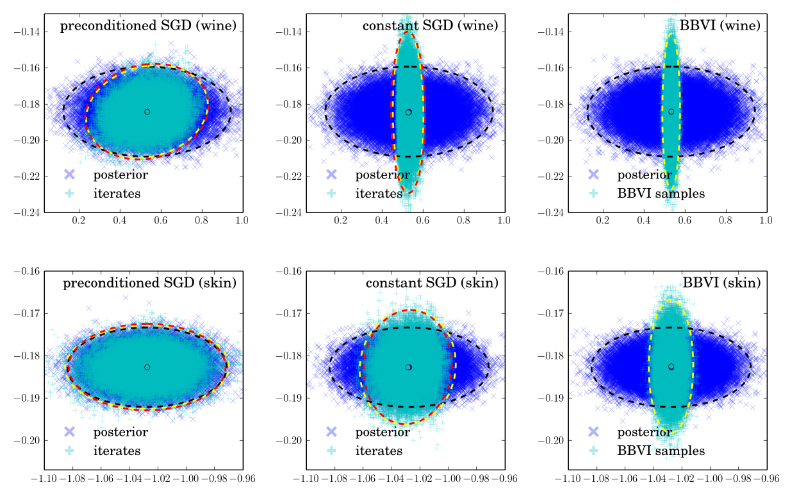
I'm not a big fan of sampling/stochastic dynamics methods (probably because most of the time I test things on neural networks), but I found this paper very enjoyable, and it makes me think I should learn more about this topic. It differs from SGLD and many other MCMC papers in that the authors didn't attempt to recover the exact posterior, but instead they did approximate SVI to keep the computations fast (although the assumptions they made are quite restrictive). There's no painstaking learning rate tuning: the paper also suggests optimal constant learning rate following the guidance of variational inference.

(Figure from the paper's ICML poster)

How does it work? Well, the authors wrote down the continuous dynamics of SGD, made a few assumptions based on CLT, quadratic approximation to the objective function near local optima, then figured out the stationary distribution $q$ of this process and optimize the learning rate as a hyper-parameter of that $q$. To be precise, let's first write down the objective function of MAP we want to minimize wrt. the model parameters $\theta$: $\mathcal{L}(\theta) = -\sum_{n=1}^N \log p(x_n|\theta) - \log p_0(\theta)$. For convenience the author considered working with $\mathcal{L}(\theta) / N$  and denote its gradient as $g(\theta)$. It's straight-forward to see that now the stochastic gradient $\hat{g}_S(\theta)$ estimated on minibatch $S$ is an unbiased estimate of $g(\theta) = \nabla \mathcal{L}(\theta) / N$, and from CLT we know that $\hat{g}_S$ is asymptotically Gaussian distributed. So here the authors make the first assumption:

(A1) $\hat{g}_S(\theta) \approx g(\theta) + \frac{1}{\sqrt{S}} \Delta g(\theta), \quad \Delta g(\theta) \sim \mathcal{N}(0; C(\theta))$

In the following are two more assumptions that when the algorithm gets close to convergence,

(A2) the noise covariance is a constant and can be decomposed, i.e. $C(\theta) = C = BB^T$; (this sounds severe but let's just assume it for simplicity)

(A3) near the local optimum the loss function $\mathcal{L}(\theta) /N$ can be well approximated with a quadratic term $\frac{1}{2}\theta^T A \theta$. (easy to derive from Taylor expansion and $A = \nabla \nabla \mathcal{L}(\theta) / N$)

Based on these assumptions the authors wrote down the continuous time stochastic differential equation of SGD as an Ornstein-Uhlenbeck process:

$d\theta(t) = -A\theta(t) dt + \sqrt{\frac{\epsilon}{S}} B dW(t)$

where $\epsilon$ is the learning rate we will optimize later. The OU process has a stationary distribution which is a Gaussian: $q(\theta) \propto \exp \left[-\frac{1}{2} \theta^T \Sigma^{-1} \theta \right]$ with the variance $\Sigma$ satisfying $\Sigma A^T + A \Sigma = \frac{\epsilon}{S}BB^T$.

Now comes the main contribution of the paper. What if we use this stationary distribution as an approximation of the true posterior? Note that $\Sigma$ is a function of matrix $A$, the mini-batch size $S$, but more importantly, the learning rate $\epsilon$. So the authors used variational inference (VI) to minimize $\mathrm{KL}[q(\theta)||p(\theta|x_1, ..., x_N)]$ wrt. $\epsilon$, and suggested running constant learning rate SGD with the minimizer $\epsilon^*$ as approximately sampling from the exact posterior. Similar procedure can be done if we use a pre-conditioning matrix $H$ (as a full or diagonal matrix) and they also worked out the optimal solutions for them. I'm not going to run through the maths here but here I just copy the solutions for interests (with $D$ dimensional data):

(constant SGD) $\epsilon^* = \frac{2DS}{N\mathcal{Tr}(BB^T)}$

(full pre-conditioned SGD) $H^* = \frac{2S}{\epsilon N}(BB^T)^{-1}$

(diagonal) $H^*_{kk} = \frac{2S}{\epsilon N (BB^T)_{kk}}$

The authors also discussed connections to Stochastic Gradient Fisher Scoring and RMSprop (I think they incorrectly claimed for Adagrad) which looks fun. But let's stop here and talk about what I think about the main results.

First we notice that $C(\theta)$ can be viewed as the empirical variance of the gradient $\hat{g}_n(\theta) = \nabla \log p(x_n|\theta)$. Now if the model is correct, then $C(\theta)$ approaches to the Fisher information matrix $I(\theta) = \mathbb{E}_x[\nabla \log p(x|\theta)^2]$ as the number of datapoint $N$ goes to infinity. Then a well known result says we can rewrite the Fisher information matrix as $I(\theta) = \mathbb{E}_x[-\nabla \nabla \log p(x|\theta)] = \lim_{N \rightarrow +\infty} \nabla \nabla \mathcal{L}(\theta) / N$. So my first guess is that if we run SGD on large datasets (we usually do) and it converges to a local optimum, then the pre-conditioned SGD with full/diagonal matrix should return very similar approximate posterior distributions to Laplace approximation/mean field VI, respectively. It's pretty easy to show them, just by substituting the optimal $H^*$ back to the constraints of $\Sigma$ and notice $BB^T \approx A$. You can do similar calculations for the constant SGD and get an isotropic Gaussian back with the precision equals to the average value of $A$'s diagonal entries.

However most of the time we know the model is wrong. In this case Laplace approximation can possible return terrible results. I think this paper might be useful for those who don't want to directly use traditional approximate inference schemes (in the cost of storing $q$ and using more parameters) and still want to get a good posterior approximation. But the performance of the SGD proposals really depend on how you actually estimate the matrix $BB^T$. Also note that case it's considered expensive to evaluate the empirical variance on the whole dataset, and instead people often use running average (see RMSprop for an example). Even if we assume the mini-batch variance is a good approximation, when the samples are hovering around, assumption (A2) doesn't hold apparently.  So the next question to ask is: can the popular adaptive learning rate schemes return some kind of approximation to the exact posterior? My experience with RMSprop says that it tends to move around the local optimum, so is it possible to get uncertainty estimates from the trajectory? And how reliable would that be? This sounds very interesting research problems and probably I need to think about it in a bit more detail.

UPDATE 11/08/16

After a happy chat with Stephan (the first author), we agreed that even when the model is wrong, the OU process predicted approximation of full-preconditioning SGD still gives you Laplace approximation (although practical simulation might disagree since the assumptions doesn't hold). My guess for the other two cases depends on that the data comes from the model.

Recently I've read an interesting paper about unsupervised learning:

The Information Sieve
Greg Ver Steeg and Aram Galstyan, ICML 2016,
http://arxiv.org/abs/1507.02284

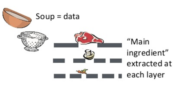
I really like the paper. In their ICML talk (shame that I didn't manage to attend!) they showed the intuition as drinking soups.

The idea is very simple. Suppose we want to learn a good representation of some observed data. Then the information sieve procedure contains two ideas. First, we should decompose the learning procedure into several stages, such that in each stage we only extract the information from the remainder of the last stage. In the soup example, the first stage gets the meat and leaves other ingredients, then the second stage gets the mushrooms from the remainders of the first stage. Second, at each stage, we want to extract as much information as possible. This depends on the functional class we use to learn representations, just like in the soup example, if the sieve size is small, then we might be able to also get the mushrooms in the first stage.

Let's go back and see the math details. The representation learning problem is formulated as correlation characterization, i.e. for data $X = (X_1, ..., X_N)$ with N components, we want to learn a representation $Y$ such that the components $X_i$ are independent with each other given $Y$. In practice we won't be able to learn such $Y$ in one stage for many problems, so why not do it recursively? Assume at stage k the input is $X^k$, where stage 0 simply has $X^0 = X$, then we repeat the following:

1. find function $f^k$ such that $Y^k = f^k(X^k)$ and $TC(X^k|Y^k)$ is minimized; $TC$ denotes "total correlation" that is defined as the KL-divergence from the joint distribution to the product of marginal distributions, which is just a multivariate version of mutual information.
2. construct remainder $X^{k+1}$ such that $X_{i}^{k+1}$ contains no information of $Y^k$, and $X^k$ can be (perfectly) reconstructed from $X^{k+1}$ and $Y^k$.

The concept of the algorithm is sound and very intriguing. I think in general we can replace step 1 with other criteria such that you can learn some representations from the input. Apparently the construction of the remainder $X^{k+1}$ depends on how we learn $Y^k$ and what we want to model in the next stage. For example we can use reconstruction loss in step 1, and extract the residuals to add in the remainder.

I was very happy with the sieve idea until I saw a confusing point in the paper. The authors emphasizes that the remainder vector $X^{k+1}$ should contain $Y^{k}$, i.e. $X^{k+1} = (X_1^{k+1}, ..., X_N^{k+1}, Y^{k})$. This sounds like you should put the meat back to the soup and drain it again. Sounds strange -- so I guess the soup example is not that appropriate. I can sort of see why this proposal is sensible, but I think in general $X^{k+1}$ just need to be a (probabilistic) function of $X^k$ and $Y^k$.

The sieve algorithm also reminds me the residual net that won ILSVRC and COCO challenges in 2015. It says we should also add a linear projection of the input to the output of the layer, i.e. $\textbf{h} = f(\textbf{x}, \textbf{W}) + \textbf{W}_{s}\textbf{x}$. Roughly speaking, the linear part $\textbf{W}_s \textbf{x}$ can be viewed as $Y^k$, and the non-linear part $f$ can be viewed as $(X_1^{k+1}, ..., X_N^{k+1})$. Does that mean we can adapt the sieve algorithm to train a residual network for unsupervised learning problems?

Before answering it, notice that the residual net uses the sum (instead of concatenation) of this two parts. So you might worry about "I'm losing something here by replacing $[\textbf{W}_s \textbf{x}, f(\textbf{x}, \textbf{W})]$ with a sum of the two", and want to work out the loss in bits. I spent some time looking at the theorems in the paper and tried to figure out, but it seems these theorems depend on the concatenation assumption and it's not clear to me how the bounds change when using summation.

However there's another way to think about this analogy. Simple calculation says that $\textbf{W}(\textbf{a} + \textbf{b}) = [\textbf{W}, \textbf{W}] [\textbf{a}^T, \textbf{b}^T]^T$. In other words, residual nets restrict the matrices that pre-multiply $Y^k$ and $f$ to be identical, and the sieve algorithm is more general here. I'm not saying you should always prefer the sieve alternative. In fact for residual networks which typically have tens or even hundreds of layers with hundreds of neurons per layer, you probably don't want to double the number of parameters just to get a bit of improvements. The original residual network paper argued its efficiency as preventing vanishing/exploding gradients when the network is very deep, which is computational. So it would be very interesting to see why residual learning helps statistically, and the sieve algorithm might be able to provide some insight here.