A Variational Analysis of Stochastic Gradient Algorithms

I've been working on approximate inference for Bayesian neural networks for quite a while. But when I talk to deep learning people, most of them say "interesting, but I still prefer back-propagation with stochastic gradient descent". Then people in the approximate inference community start to think about how to link SGD to approximate inference, and in this line a very recent paper catched my eyes:

A Variational Analysis of Stochastic Gradient Algorithms
Stephan Mandt, Matt Hoffman, and David Blei, ICML 2016
http://jmlr.org/proceedings/papers/v48/mandt16.pdf

I'm not a big fan of sampling/stochastic dynamics methods (probably because most of the time I test things on neural networks), but I found this paper very enjoyable, and it makes me think I should learn more about this topic. It differs from SGLD and many other MCMC papers in that the authors didn't attempt to recover the exact posterior, but instead they did approximate SVI to keep the computations fast (although the assumptions they made are quite restrictive). There's no painstaking learning rate tuning: the paper also suggests optimal constant learning rate following the guidance of variational inference.

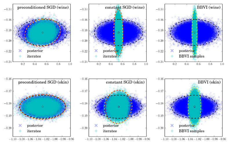
(Figure from the paper's ICML poster)

How does it work? Well, the authors wrote down the continuous dynamics of SGD, made a few assumptions based on CLT, quadratic approximation to the objective function near local optima, then figured out the stationary distribution $q$ of this process and optimize the learning rate as a hyper-parameter of that $q$. To be precise, let's first write down the objective function of MAP we want to minimize wrt. the model parameters $\theta$: $\mathcal{L}(\theta) = -\sum_{n=1}^N \log p(x_n|\theta) - \log p_0(\theta)$. For convenience the author considered working with $\mathcal{L}(\theta) / N$  and denote its gradient as $g(\theta)$. It's straight-forward to see that now the stochastic gradient $\hat{g}_S(\theta)$ estimated on minibatch $S$ is an unbiased estimate of 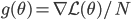$g(\theta) = \nabla \mathcal{L}(\theta) / N$, and from CLT we know that $\hat{g}_S$ is asymptotically Gaussian distributed. So here the authors make the first assumption:

(A1) 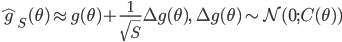$\hat{g}_S(\theta) \approx g(\theta) + \frac{1}{\sqrt{S}} \Delta g(\theta), \quad \Delta g(\theta) \sim \mathcal{N}(0; C(\theta))$

In the following are two more assumptions that when the algorithm gets close to convergence,

(A2) the noise covariance is a constant and can be decomposed, i.e. 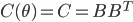$C(\theta) = C = BB^T$; (this sounds severe but let's just assume it for simplicity)

(A3) near the local optimum the loss function $\mathcal{L}(\theta) /N$ can be well approximated with a quadratic term $\frac{1}{2}\theta^T A \theta$. (easy to derive from Taylor expansion and $A = \nabla \nabla \mathcal{L}(\theta) / N$)

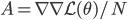Based on these assumptions the authors wrote down the continuous time stochastic differential equation of SGD as an Ornstein-Uhlenbeck process:

$d\theta(t) = -A\theta(t) dt + \sqrt{\frac{\epsilon}{S}} B dW(t)$

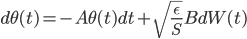
where $\epsilon$ is the learning rate we will optimize later. The OU process has a stationary distribution which is a Gaussian: $q(\theta) \propto \exp \left[-\frac{1}{2} \theta^T \Sigma^{-1} \theta \right]$ with the variance $\Sigma$ satisfying $\Sigma A^T + A \Sigma = \frac{\epsilon}{S}BB^T$.

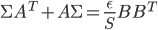Now comes the main contribution of the paper. What if we use this stationary distribution as an approximation of the true posterior? Note that $\Sigma$ is a function of matrix $A$, the mini-batch size $S$, but more importantly, the learning rate $\epsilon$. So the authors used variational inference (VI) to minimize $\mathrm{KL}[q(\theta)||p(\theta|x_1, ..., x_N)]$ wrt. $\epsilon$, and suggested running constant learning rate SGD with the minimizer $\epsilon^*$ as approximately sampling from the exact posterior. Similar procedure can be done if we use a pre-conditioning matrix $H$ (as a full or diagonal matrix) and they also worked out the optimal solutions for them. I'm not going to run through the maths here but here I just copy the solutions for interests (with $D$ dimensional data):

(constant SGD) 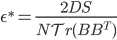$\epsilon^* = \frac{2DS}{N\mathcal{Tr}(BB^T)}$

(full pre-conditioned SGD) 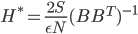$H^* = \frac{2S}{\epsilon N}(BB^T)^{-1}$

(diagonal) 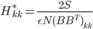$H^*_{kk} = \frac{2S}{\epsilon N (BB^T)_{kk}}$

The authors also discussed connections to Stochastic Gradient Fisher Scoring and RMSprop (I think they incorrectly claimed for Adagrad) which looks fun. But let's stop here and talk about what I think about the main results.

First we notice that $C(\theta)$ can be viewed as the empirical variance of the gradient $\hat{g}_n(\theta) = \nabla \log p(x_n|\theta)$. Now if the model is correct, then $C(\theta)$ approaches to the Fisher information matrix $I(\theta) = \mathbb{E}_x[\nabla \log p(x|\theta)^2]$ as the number of datapoint $N$ goes to infinity. Then a well known result says we can rewrite the Fisher information matrix as $I(\theta) = \mathbb{E}_x[-\nabla \nabla \log p(x|\theta)] = \lim_{N \rightarrow +\infty} \nabla \nabla \mathcal{L}(\theta) / N$. So my first guess is that if we run SGD on large datasets (we usually do) and it converges to a local optimum, then the pre-conditioned SGD with full/diagonal matrix should return very similar approximate posterior distributions to Laplace approximation/mean field VI, respectively. It's pretty easy to show them, just by substituting the optimal $H^*$ back to the constraints of $\Sigma$ and notice $BB^T \approx A$. You can do similar calculations for the constant SGD and get an isotropic Gaussian back with the precision equals to the average value of $A$'s diagonal entries.

However most of the time we know the model is wrong. In this case Laplace approximation can possible return terrible results. I think this paper might be useful for those who don't want to directly use traditional approximate inference schemes (in the cost of storing $q$ and using more parameters) and still want to get a good posterior approximation. But the performance of the SGD proposals really depend on how you actually estimate the matrix $BB^T$. Also note that case it's considered expensive to evaluate the empirical variance on the whole dataset, and instead people often use running average (see RMSprop for an example). Even if we assume the mini-batch variance is a good approximation, when the samples are hovering around, assumption (A2) doesn't hold apparently.  So the next question to ask is: can the popular adaptive learning rate schemes return some kind of approximation to the exact posterior? My experience with RMSprop says that it tends to move around the local optimum, so is it possible to get uncertainty estimates from the trajectory? And how reliable would that be? This sounds very interesting research problems and probably I need to think about it in a bit more detail.

 

UPDATE 11/08/16

After a happy chat with Stephan (the first author), we agreed that even when the model is wrong, the OU process predicted approximation of full-preconditioning SGD still gives you Laplace approximation (although practical simulation might disagree since the assumptions doesn't hold). My guess for the other two cases depends on that the data comes from the model.