Recently I've read an interesting paper about unsupervised learning:
The Information Sieve
Greg Ver Steeg and Aram Galstyan, ICML 2016,
http://arxiv.org/abs/1507.02284
I really like the paper. In their ICML talk (shame that I didn't manage to attend!) they showed the intuition as drinking soups.
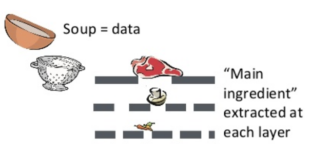
The idea is very simple. Suppose we want to learn a good representation of some observed data. Then the information sieve procedure contains two ideas. First, we should decompose the learning procedure into several stages, such that in each stage we only extract the information from the remainder of the last stage. In the soup example, the first stage gets the meat and leaves other ingredients, then the second stage gets the mushrooms from the remainders of the first stage. Second, at each stage, we want to extract as much information as possible. This depends on the functional class we use to learn representations, just like in the soup example, if the sieve size is small, then we might be able to also get the mushrooms in the first stage.
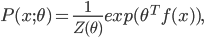
Let's go back and see the math details. The representation learning problem is formulated as correlation characterization, i.e. for data  with N components, we want to learn a representation
  such that the components
  are independent with each other given . In practice we won't be able to learn such in one stage for many problems, so why not do it recursively? Assume at stage k the input is
  , where stage 0 simply has
  , then we repeat the following:
- find function
 such that
  and
and  is minimized;
  denotes "total correlation" that is defined as the KL-divergence from the joint distribution to the product of marginal distributions, which is just a multivariate version of mutual information.
 - construct remainder
 such that
  contains no information of
  , and can be (perfectly) reconstructed from and .
The concept of the algorithm is sound and very intriguing. I think in general we can replace step 1 with other criteria such that you can learn some representations from the input. Apparently the construction of the remainder depends on how we learn and what we want to model in the next stage. For example we can use reconstruction loss in step 1, and extract the residuals to add in the remainder.
I was very happy with the sieve idea until I saw a confusing point in the paper. The authors emphasizes that the remainder vector should contain  , i.e.
  . This sounds like you should put the meat back to the soup and drain it again. Sounds strange -- so I guess the soup example is not that appropriate. I can sort of see why this proposal is sensible, but I think in general just need to be a (probabilistic) function of and .
The sieve algorithm also reminds me the residual net that won ILSVRC and COCO challenges in 2015. It says we should also add a linear projection of the input to the output of the layer, i.e.  . Roughly speaking, the linear part
  can be viewed as , and the non-linear part
  can be viewed as
  . Does that mean we can adapt the sieve algorithm to train a residual network for unsupervised learning problems?
Before answering it, notice that the residual net uses the sum (instead of concatenation) of this two parts. So you might worry about "I'm losing something here by replacing ![[\textbf{W}_s \textbf{x}, f(\textbf{x}, \textbf{W})]](http://www.yingzhenli.net/home/blog/wp-content/plugins/latex/cache/tex_de056466e2af0f1a1b14af9ca4413413.gif) with a sum of the two", and want to work out the loss in bits. I spent some time looking at the theorems in the paper and tried to figure out, but it seems these theorems depend on the concatenation assumption and it's not clear to me how the bounds change when using summation.
with a sum of the two", and want to work out the loss in bits. I spent some time looking at the theorems in the paper and tried to figure out, but it seems these theorems depend on the concatenation assumption and it's not clear to me how the bounds change when using summation.
However there's another way to think about this analogy. Simple calculation says that ![\textbf{W}(\textbf{a} + \textbf{b}) = [\textbf{W}, \textbf{W}] [\textbf{a}^T, \textbf{b}^T]^T](http://www.yingzhenli.net/home/blog/wp-content/plugins/latex/cache/tex_ef5b3439cb08d522eba7459de095dccd.gif) . In other words, residual nets restrict the matrices that pre-multiply and to be identical, and the sieve algorithm is more general here. I'm not saying you should always prefer the sieve alternative. In fact for residual networks which typically have tens or even hundreds of layers with hundreds of neurons per layer, you probably don't want to double the number of parameters just to get a bit of improvements. The original residual network paper argued its efficiency as preventing vanishing/exploding gradients when the network is very deep, which is computational. So it would be very interesting to see why residual learning helps statistically, and the sieve algorithm might be able to provide some insight here.
. In other words, residual nets restrict the matrices that pre-multiply and to be identical, and the sieve algorithm is more general here. I'm not saying you should always prefer the sieve alternative. In fact for residual networks which typically have tens or even hundreds of layers with hundreds of neurons per layer, you probably don't want to double the number of parameters just to get a bit of improvements. The original residual network paper argued its efficiency as preventing vanishing/exploding gradients when the network is very deep, which is computational. So it would be very interesting to see why residual learning helps statistically, and the sieve algorithm might be able to provide some insight here.


![\mathrm{I}[s; x] = \mathrm{KL}[\tilde{p}(s, x) || \tilde{p}(s) \tilde{p}(x)].](http://www.yingzhenli.net/home/blog/wp-content/plugins/latex/cache/tex_6df580dac667590c769263154aeb8030.gif)
![\mathrm{I}[s; x] = 0](http://www.yingzhenli.net/home/blog/wp-content/plugins/latex/cache/tex_e87ff28cb7ffaf246198a72d6f20c21e.gif)


![\mathcal{L}[p; q] = \mathrm{I}[s; x] - \mathbb{E}_{\tilde{p}(x)}[\mathrm{KL}[\tilde{p}(s|x) ||q(s|x)] \\ = \mathrm{H}[s] + \mathbb{E}_{\tilde{p}(s, x)}[\log q(s|x)].](http://www.yingzhenli.net/home/blog/wp-content/plugins/latex/cache/tex_decb1089977e52be6fc2bce1e1855d00.gif)


![\tilde{p}(s = 0) \mathbb{E}_{p(x)}[\log (1 - q(s = 1|x))] + \tilde{p}(s = 1) \mathbb{E}_{p_D(x)}[\log q(s = 1|x)].](http://www.yingzhenli.net/home/blog/wp-content/plugins/latex/cache/tex_2c99d61db085ecd2fe04b6bc75ee3bbe.gif)

![\mathcal{L}[p; q]](http://www.yingzhenli.net/home/blog/wp-content/plugins/latex/cache/tex_50c4f2863f9574f34d584c74904de0c6.gif)
![\mathrm{I}[s; x]](http://www.yingzhenli.net/home/blog/wp-content/plugins/latex/cache/tex_f610b226722573201d0d6e6bd94c0da3.gif)
![\mathrm{JS}[p(x)||p_D(x)]](http://www.yingzhenli.net/home/blog/wp-content/plugins/latex/cache/tex_83f74baf9d6ce987f9a5e314fa142434.gif)

![k \in [1, N]](http://www.yingzhenli.net/home/blog/wp-content/plugins/latex/cache/tex_cd7f1d1b3c099f29059a3754da09ad1c.gif)

![\exists k' \in [1, N] s.t. f_{k'}(x) = f_{k'}(T(x)), \forall x \in \{x_i\}.](http://www.yingzhenli.net/home/blog/wp-content/plugins/latex/cache/tex_2103f9b7f0608d259c98925b088a1697.gif)