Here's a general case that the 1-step learning will failed to achieve the optimal parameters, inspired by [1].
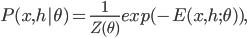
Consider the exponential family model
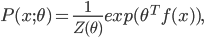
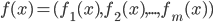 (we can also consider it as a multi-expert system). Assume the variable
  takes discrete states and a transition operator
  s.t. for any , there exists an integer
 ![k \in [1, N]](http://www.yingzhenli.net/home/blog/wp-content/plugins/latex/cache/tex_cd7f1d1b3c099f29059a3754da09ad1c.gif) such that
such that 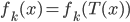 . Then we can find some data set
  satisfying
 ![\exists k' \in [1, N] s.t. f_{k'}(x) = f_{k'}(T(x)), \forall x \in \{x_i\}.](http://www.yingzhenli.net/home/blog/wp-content/plugins/latex/cache/tex_2103f9b7f0608d259c98925b088a1697.gif)
 , which means that we cannot achieve the optimum as the maximum likelihood algorithm does.
The statement indicates that the performance of the one-step learning depends on the model distribution and the transition in each step of the Markov chain. However, though the failure above will be addressed if provided enough training data points, in some cases the parameters will never converge or converge to the other points rather than the ML result. See the cases of noisy swirl operator and noisy star trek operator in [1] for details. But fortunately, training energy models with sampling from factored likelihood and posterior in each step yields good results with CD-k, which will be explained below.
Let's consider the justification of the CD-k algorithm Rich and I discussed in our meeting, to answer the questions I raised in the last research note. We learn the energy models by the maximum likelihood method, i.e. maximize

 is our constructed (optimal) model and
  is the data distribution. It's easy to see
 . For the energy model with coefficients
  we have
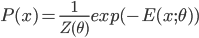
 is differentiable w.r.t. and
  is some normalizer. Then by doing some math we get the derivative of the expectation of the log-likelihood w.r.t. as follows:

In the RBM case, we have the model joint distribution

However, the expectation is intractable, and in practice we sample the training set  from . In this case we approximate the first term of the derivative by
 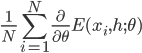 , where
  equals to, or is sampled from, the conditional distribution
  . For better generalization, we don't want the ML algorithm to minimize the KL-divergence exactly to 0, as P will be the average of Dirac functions
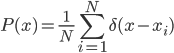
which makes the probability be zero at the points other than those in the training set. That's why the approximation of the ML optimum can help to smooth the model distribution.
Also notice that the derivative of the log-likelihood of the RBM contains the expectation of the energy function over both and with the joint distribution  , which is also intractable. In general we use the samples from some MCMC method, e.g. Gibbs sampling, to approximate that derivative. Without loss of generality we assume
  have discrete states and the Markov chain is aperiodic, then consider the sampling conditional probability
  and
and  , the Gibbs chain will converge to the equilibrium distribution
  and
and  . To specify the statement, consider

 and
and  , then we have
 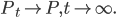 So that justify the truncating of the Gibbs train after k full-step sampling, and Hinton asserted that experiments showed that k = 1 yielded good training results.
References
[1] David J. C. MacKay, Failures of the One-Step Learning Algorithm, 2001.